Mini Project 2: Computational Art
Due: 10:30 am, Tue 25 FebPreliminaries
Introduction
The idea of this assignment is to create art using computation as an artistic medium. As you saw in class, there are a ton of interesting ways to combine computation and art. In this assignment you will be exploring one particular means of using computers to generate images. We also encourage you to think about what “computational creativity” is, what it means to create art computationally, how it differs from art in the traditional sense, and how it fits in today’s society.
For the “going beyond” portion you will have the opportunity to extend your work by exploring topics such as computational generation of movies and real-time visualization of auditory signals.
Acknowledgments
This assignment has been adapted from Harvey Mudd Professor Chris Stone’s assignment posted at the Stanford Nifty Assignments collection.
Skills Emphasized
- Recursion
- Working with color
- Randomness
- Creating Images
- Creating Movies [for the going beyond portion]
- Auditory Visualization [for the going beyond portion]
Computational Creativity
At some point in your mathematical career you have probably seen a figure that looks like this:
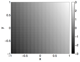
This is a graphical representation of the function f(x, y) = 2x + y where the brightness of each position in the figure above represents the value of the function evaluated at a particular (x, y) pair (note the bar on the side that translates between brightness and the numerical value of the function).
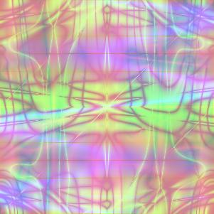
From a visual point of view, this figure doesn’t look particularly rich. However, for more complex functions things start to get more interesting. Here is a plot of the function f(x, y) = sin(10pi*xy)
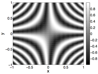
Things get even more interesting when we use the power of computation to generate functions by randomly composing elementary functions with each other. Here is a plot of the randomly generated function f(x, y) = cos(pi*((cos(pi*sin(pi*(((x+y)/2*cos(pi*y))+cos(pi*cos(pi*y)))/2))*((((cos(pi*y)+(x*y))/2*(cos(pi*y)*sin(pi*x)))+sin(pi*((x+x)/2+cos(pi*y))/2))/2*sin(pi*sin(pi*sin(pi*(y+y)/2)))))+sin(pi*(cos(pi*cos(pi*cos(pi*sin(pi*x))))+sin(pi*sin(pi*((x*x)*sin(pi*y)))))/2))/2)
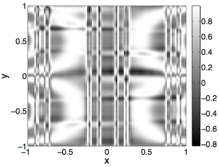
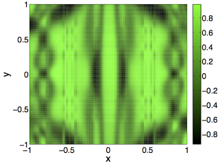
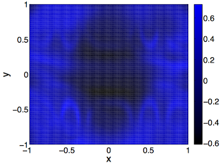
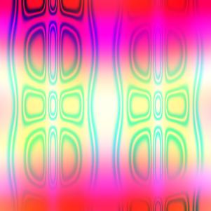
Cool! Next, we bring in the idea of color. Instead of generating one random function, we generate three (one for each of the color channels red, green, and blue). Here are 3 figures representing randomly generated functions for each of the color channels. (Note: in a slight change of notation we are now using the function avg(x, y) instead of (x + y) / 2.)
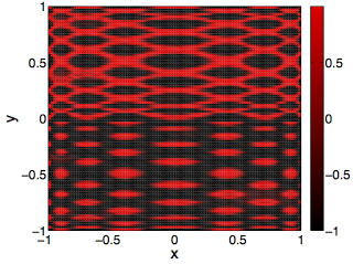
red(x, y) = sin(pi * avg((((cos(pi * (sin(pi * cos(pi * y)) * avg(avg(x, x),
sin(pi * y)))) * avg(sin(pi * (sin(pi * y) * (y * x))), cos(pi * cos(pi * (y *
y))))) * sin(pi * (sin(pi * (sin(pi * y) * sin(pi * y))) * cos(pi * ((y * y) *
sin(pi * y)))))) * sin(pi * avg(cos(pi * avg(((y * x) * (x * x)), sin(pi * (y
* x)))), sin(pi * avg(avg(sin(pi * x), avg(x, x)), sin(pi * avg(x, y))))))),
cos(pi * cos(pi * avg(sin(pi * sin(pi * avg((x * x), (x * x)))), sin(pi *
sin(pi * sin(pi * sin(pi * y)))))))))
green(x, y) = sin(pi * ((avg(avg(cos(pi * (cos(pi * cos(pi * x)) * (cos(pi * x)
* avg(y, x)))), ((cos(pi * cos(pi * y)) * (cos(pi * x) * (x * y))) * sin(pi *
sin(pi * avg(y, y))))), cos(pi * (avg(sin(pi * sin(pi * x)), sin(pi * sin(pi *
x))) * sin(pi * sin(pi * (x * y)))))) * avg((avg(cos(pi * sin(pi * cos(pi *
x))), avg((sin(pi * x) * cos(pi * y)), avg(cos(pi * x), cos(pi * x)))) *
avg(avg(sin(pi * cos(pi * x)), sin(pi * sin(pi * x))), (avg(cos(pi * x),
avg(y, x)) * avg(sin(pi * y), sin(pi * x))))), (cos(pi * cos(pi * (avg(y, y) *
(y * x)))) * cos(pi * cos(pi * sin(pi * avg(x, x))))))) * sin(pi *
avg(avg(sin(pi * cos(pi * sin(pi * cos(pi * x)))), avg(sin(pi * cos(pi *
cos(pi * y))), ((sin(pi * y) * (x * y)) * cos(pi * (y * y))))), cos(pi *
avg(((cos(pi * y) * (y * y)) * avg(sin(pi * y), cos(pi * y))), (((x * x) *
avg(y, x)) * cos(pi * sin(pi * x)))))))))
blue(x, y) = avg(sin(pi * (avg(cos(pi * avg((cos(pi * (x * x)) * cos(pi * (x *
y))), avg(avg((x * x), avg(y, y)), avg(cos(pi * y), cos(pi * x))))),
avg(avg(avg((sin(pi * y) * (x * y)), sin(pi * (x * x))), avg(((x * x) * sin(pi
* y)), (avg(x, x) * sin(pi * y)))), avg((cos(pi * sin(pi * y)) * cos(pi *
avg(x, x))), sin(pi * avg(sin(pi * y), sin(pi * y)))))) * cos(pi *
avg(avg(avg(sin(pi * (x * x)), avg(sin(pi * y), sin(pi * x))), cos(pi *
avg(cos(pi * y), avg(y, x)))), (((avg(x, y) * cos(pi * x)) * cos(pi * avg(y,
x))) * avg(cos(pi * (y * x)), ((x * x) * (y * x)))))))), avg(((((sin(pi *
sin(pi * avg(x, x))) * avg(avg(sin(pi * y), sin(pi * y)), avg(avg(x, x),
cos(pi * y)))) * sin(pi * sin(pi * sin(pi * (y * y))))) * avg(cos(pi *
avg(avg(avg(x, y), (y * x)), cos(pi * sin(pi * x)))), (sin(pi * sin(pi *
sin(pi * x))) * cos(pi * ((y * y) * cos(pi * x)))))) * avg(cos(pi * cos(pi *
sin(pi * cos(pi * avg(x, y))))), (sin(pi * (cos(pi * avg(y, x)) * sin(pi *
cos(pi * x)))) * ((sin(pi * cos(pi * y)) * avg(avg(x, x), cos(pi * x))) *
avg((sin(pi * x) * avg(y, x)), sin(pi * sin(pi * x))))))), ((cos(pi * cos(pi *
(sin(pi * (y * y)) * cos(pi * cos(pi * x))))) * avg(sin(pi * avg(cos(pi *
sin(pi * y)), (cos(pi * x) * avg(x, x)))), cos(pi * cos(pi * cos(pi * avg(x,
y)))))) * sin(pi * (avg((cos(pi * (y * y)) * cos(pi * sin(pi * y))), avg(((x *
x) * sin(pi * x)), cos(pi * sin(pi * y)))) * avg(sin(pi * (avg(y, x) * avg(x,
x))), cos(pi * avg((y * y), avg(y, y)))))))))
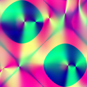
Of course the real fun is when we put all of these individual color channel images together into a single image.
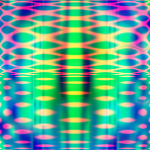
Voila! Computational creativity (there are some deep philosophical issues behind whether this can be called creativity… We don’t pretend to know the answers, but we do think that these pictures look really cool!)
- Why Love Generative Art?
- Is Art created by AI Really Art?
- Robot Art Raises Questions About Human Creativity
- Afrofuturist Artist Creates Stunning Portraits of Black Artists With Deep Dream AI Algorithms
- Vincent van Bot: the robots turning their hand to art
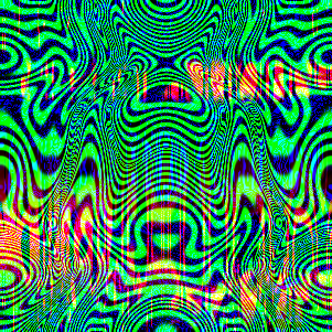
Here are some other examples taken from students who have done this assignment at Harvey Mudd:
Part 0: Install and test Python Imaging Library
To get started on the assignment:
- Click on the invitation link at https://classroom.github.com/a/4fTu6p3c
- Accept the assignment and follow the instructions to get to your repository page, which looks something like https://github.com/sd2020spring/ComputationalArt-myname
- Clone the repository to your computer. The starter code is in
recursive_art.py.
In addition to fetching the starter code, you should also install the Pillow fork of the Python Imaging Library (“PIL”). To do so, execute the following command at the Linux terminal:
$ conda install Pillow
The starter code includes a function called test_image that uses PIL to
generate an image where each pixel has a random color value. When you run the
starter code, you should see several unit test failures from functions you
will implement later, and it should save an image file named noise.png in
your run directory. You can view noise.png using the built-in tool
Image Viewer (eog on the command line).
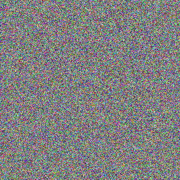
While this looks pretty cool (and it might be fun to convince your gullible friends it is a Magic Eye picture), I wouldn’t call it art. In the rest of the assignment, you will combine randomness with structure to produce more compelling images.
Once you’ve verified that PIL is working correctly, comment out the line that
calls test_image and un-comment the line that calls generate_art. If you
run into errors installing Pillow or generating the test image, talk to a
NINJA.
Part 1: Understanding the structure of the starter code and making your first image
First, make sure you are familiar with the starter code and how it utilizes
the PIL library to generate a simple image. The relevant code is in the
generate_art function:
# Functions for red, green, and blue channels - where the magic happens!
red_function = ["x"]
green_function = ["y"]
blue_function = ["x"]

# Create image and loop over all pixels
im = Image.new("RGB", (x_size, y_size))
pixels = im.load()
for i in range(x_size):
    for j in range(y_size):
        x = remap_interval(i, 0, x_size, -1, 1)
        y = remap_interval(j, 0, y_size, -1, 1)
        pixels[i, j] = (
            color_map(evaluate_random_function(red_function, x, y)),
            color_map(evaluate_random_function(green_function, x, y)),
            color_map(evaluate_random_function(blue_function, x, y)))

im.save(filename)
The arguments to this function are a string filename where the image file
will be saved, and two optional arguments x_size and y_size which set the
image dimensions in pixels. If the size arguments are not given, they default
to 350.
Let’s look at the code line-by-line and make sure we understand what is happening
red_function = ["x"]
green_function = ["y"]
blue_function = ["x"]
For testing purposes we are going to generate the red channel with the function x, the green channel with the function y, and the blue channel with the function x. Eventually we will do more complex things as in the examples above, but this will allow us to get started.
im = Image.new("RGB", (x_size, y_size))
pixels = im.load()
In this code, we are creating a new image with the given size. The input “RGB”
indicates that the image has three color channels which are in order “red”,
“green”, and “blue”. The im.load command returns a pixel access object that
we can use to set the color values in our new image.
for i in range(x_size):
    for j in range(y_size):
These lines create a nested loop in which we will set each pixel value based on evaluating the red, green, and blue channel functions.
        x = remap_interval(i, 0, x_size, -1, 1)
        y = remap_interval(j, 0, y_size, -1, 1)
These lines are necessary because the functions we will be generating (as in
the examples above) have inputs in the interval [-1, +1] and outputs in the
interval [-1, +1]. If we were to simply input the raw pixel coordinates, these
would go from [0, 349]. The remap_interval function (which you will
implement) transforms the pixel index (which is in [0, 349]) to the interval we
want ([-1, +1]).
        pixels[i, j] = (
            color_map(evaluate_random_function(red_function, x, y)),
            color_map(evaluate_random_function(green_function, x, y)),
            color_map(evaluate_random_function(blue_function, x, y)))
This code evaluates each the red, green, and blue channel functions to obtain
the intensity for each color channel for the pixel (i, j). We need to use the
color_map function (which calls your remap_interval function) since the
color channel function outputs are floats in [-1, +1], but PIL expects the
color intensity values to be integers in the range [0, 255].
im.save(filename)
This final line saves your image to disk as the specified filename (which will
be "myart.png" if you don’t change it). You can view myart.png using the
built-in tool image_viewer.
The initial starter code will not work without modification. To get started and generate your first image, you will need to make the following modifications:
- Implement
remap_interval. To help you get started we have defined several doctests and filled out the docstring. - Modify the function
evaluate_random_functionso that if the function [“x”] is passed in, the input argument x is returned, and if the function [“y”] is passed in, the input argument y is returned. To help you understand this, we have added two doctests demonstrating the behavior your function should have.
If you have done everything properly, when you run your code you shouldn’t get
any doctest failure messages and an image file will show up in your
computational_art folder called myart.png. The image should look like this:

Part 2: Generating and evaluating random recursive functions
Now that you have created your first image, you should start filling out the
function build_random_function. As you fill in this function, you will also
want to modify your evaluate_random_function method so that it can handle
the recursive functions that build_random_function is generating.
In order to be able to see the images your code is generating as you make
these changes, you should overwrite the simple function values for red, green,
and blue in the body of generate_art with random functions generated with
minimum depth 7 and maximum depth 9 (definitely play around with other depths
for really cool effects though). The modified code should look like this:
red_function = build_random_function(7, 9)
green_function = build_random_function(7, 9)
blue_function = build_random_function(7, 9)
We will be representing function composition using nested lists. Here is a scheme for representing function compositions using a list:
["elementary function name here", argument 1 (optional), argument 2 (optional)]
For instance, to represent the function f(x, y) = x we would use (you have already seen this in the first part of the assignment):
["x"]
Since the function f(x, y) = x has no additional arguments, the 2nd and 3rd elements of the list have been omitted. Note, that the string “x” has no special meaning to Python, in the first part of the assignment you had to tell Python how to evaluate this function for a particular input pair (x, y).
Alternatively, consider the following list representation of the function f(x, y) = sin(pi * x)
["sin_pi", ["x"]]
In contrast to the function f(x, y) = x, here we use the second list element to
specify the function that we are going to compose with sin_pi.
Next, consider the following representation of the function f(x, y) = xy
["prod", ["x"], ["y"]]
In this example we used both the second and third element to specify the two arguments to the prod function.
To create more complex functions we use more deeply-nested lists. For instance, f(x, y) = sin(pix)cos(pi*x) would be represented as:
["prod", ["sin_pi", ["x"]], ["cos_pi", ["x"]]]
Implement the function build_random_function in the provided Python file
recursive_art.py.
The two input arguments to build_random_function are min_depth and
max_depth. The input min_depth specifies the minimum amount of nesting for
the function that you generate (the depth of the preceding examples are 2 and
3 respectively). The input max_depth specifies the maximum amount of nesting
of the function that you generate. To help better understand the idea of the
depth of the function the following diagram might help:
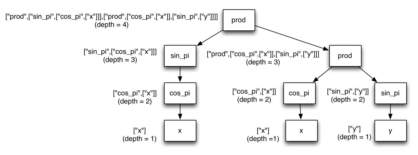
Click image to enlarge
In this figure the nested function is represented as a tree. The elementary
functions are represented in the label on the relevant box, and an arrow from
box i to box j indicates that the function represented by box j is an argument
to the function represented by box i. To the left of each box is the list
representation of the function (notice that the list representation includes
the function representation of the functions that it points to). Also to the
left of the box is the depth of the function (i.e. the degree of nested-ness of
the list representation). The min_depth and max_depth inputs, refer to the
depths listed in the figure above.
Your build_random_function implementation should create random functions
from the following required building blocks:
prod(a, b) = abavg(a, b) = 0.5*(a + b)cos_pi(a) = cos(pi * a)sin_pi(a) = sin(pi * a)x(a, b) = ay(a, b) = b
The key characteristic of each of these building blocks is that provided each
of the inputs specified to the function is in the range [-1, 1] then the output
of the function will also be in the range [-1, 1]. In addition to the required
functions above, add two additional function building blocks that have the
crucial property that if the inputs to the function are between [-1, 1] the
output will also be in the interval [-1, 1]. As part of creating
build_random_function you should add an appropriate docstring. You may also
want to add additional doctests. Your implementation of
build_random_function should make heavy use of the principle of
recursion.
As stated before, as you modify build_random_function you will also want to
modify the implementation of evaluate_random_function that you created in Part 1.
In order to complete the required part of the assignment, your
evaluate_random_function must be able to evaluate any random function
generated by build_random_function.
Going Beyond
There are a number of interesting directions to take this assignment.
Extension 1: Lambda Functions!
Explore the use of lambda functions to
represent deeply nested compositions of functions. For this extension you
should replace the list representation of nested functions with lambda
functions. For instance, ["cos_pi", ["prod", ["x", "y"]]] would be
represented as the lambda function:
lambda x, y: cos(pi * (lambda x, y: (lambda x, y: x)(x, y) * (lambda x, y: y)(x, y))(x, y)).
Using lambda functions will allow you to return a variable of type function
from your build_random_function code. In order to evaluate the function at
a particular (x, y) pair all you have to do is pass (x, y) into your function
variable (this obviates the need for evaluate_random_function). For
instance,
green = build_random_function(7, 9)
green_channel_pixel_for_x_y = green(x, y)
Extension 2: Movies!!!
Instead of building random functions of two variables (x, y) build random function of three variables (x, y, t) where t represents the frame number in a movie rescaled to the interval [-1, +1]. The easiest way to create these movies is to output a series of image files (one for each frame of the movie) and then use a command line tool such as avconv to encode them into a movie.
For instance, if you created images frame001.png, frame002.png, …,
frame100.png you could encode these images into a movie using the following
command in Linux (assuming you have already installed avconv via apt-get).
$ avconv -i frame%03d.png -vb 20M mymovie.avi
Use frame%03d.png if your files are named e.g. frame001.png, frame002.png,
frame003.png. Use frame%d.png if your files are named e.g. frame%03d.png,
frame2.png, frame3.png.
If you want to do something cleaner, you should investigate some libraries for
actually creating the movie within Python itself - e.g., moviepy (removing the need for saving
the frames individually and running avconv). You can also use the Python
subprocess library to call
avconv from within Python, although in this case you still need to save
the individual frames.
The results are pretty cool! Check out these examples that I created (Note: for these examples I ran the time variable from -1 to 1 and then in reverse from 1 to -1):
Extension 3: Pulsating Music Visualizer!!!!!
The idea here will be to have a visualization that responds in real-time to loudness changes as picked up by your computer’s microphone. This can be used to have a visual that pulses along to the music (or your voice).
Linux: In order to process audio from the microphone, check out pyalsaaudio. To use the library you will need to install both the pyalsaaudio package and some libraries that it depends on. Here are the install commands:
$ apt-get install libasound2-dev
$ pip install pyalsaaudio
Here is some simple code for getting audio from the mic and displaying the volume:
import alsaaudio
import audioop

inp = alsaaudio.PCM(alsaaudio.PCM_CAPTURE, 0)
inp.setchannels(1)
inp.setrate(16000)
inp.setformat(alsaaudio.PCM_FORMAT_S16_LE)
inp.setperiodsize(160)

while True:
    l, data = inp.read()
    if l:
        print(audioop.rms(data, 2))
To display images in real-time (as opposed to using an image viewer to checkout the images after you have saved them to a file), I recommend using pygame. To install pygame, follow the instructions from the recipe page.
One very important thing is that your code will not be fast enough to generate the appropriate image for a given volume level in real-time. You should generate the images for various volume levels ahead of time, and have them loaded and ready to be displayed using pygame when appropriate.
Project Reflection
Please prepare a short document (~1 paragraph to 1-2 pages) that addresses:
From a process point of view, what went well? What could you improve? Other possible reflection topics: Was your project appropriately scoped? Did you have a good plan for unit testing? How will you use what you learned going forward? What do you wish you knew before you started that would have helped you succeed?
What are your thoughts on “computational creativity”? Possible reflection topics for this: How creative do you believe you were in making your art? How do you think computational art differs from more traditional art? Who might deserve credit for the creation of your final piece of computational art?
Add your Reflection to your GitHub repository. This can be in the form of:
- a Markdown file, or
- a Jupyter notebook, or
- a PDF document, or
Turning in your assignment
In order to turn in your assignment, you will need to push your code to GitHub
(for the main assignment, all code will be in recursive_art.py.
Submit a link on Canvas to your recursive_art.py on GitHub.
If you
choose to do the going beyond portion, it is up to you how you structure your
code for that portion). You should also push at least two images generated by
your program using the file names example1.png and example2.png (if
you don’t want to use PNG, feel free to use a different standard image
format).
Optional in-class Gallery Show
We will be creating an art gallery of examples from the class.
To participate,
submit your art files (either images or movies) by email to the instructors along with a brief file
called ARTIST_STATEMENT.txt that contains:
- Your name (if not anonymous)
- The additional functions you used to create the artwork (beyond the basic set of
prod,cos, …) - An artist’s statement explaining your work of art.
The types of things you might want to touch on in the artist statement are:
- What is the title of your composition?
- What are the major themes explored in your piece?
- What are your major influences as an artist that lead you to create this piece?
A much better and more extensive list of guidance around producing an artist’s statement can be found here.
In order to make it into the exhibition you should submit your art no later than: Mon, Feb 24.